Random Machine Learning Theory

Just my personal notes!

Self-Supervised Learning

Contrastive Loss

• The goal of contrastive representation learning is to learn such an embedding space in which similar sample pairs stay close to each other while dissimilar ones are far apart
• Key Ingredients
  • Heavy Data Augmentations
  • Large Batch Size
  • Hard Negative Mining

Semi-Supervised Learning

(Some tricks from UDA…) Training Signal Annealing for Low-data Regime. In semi-supervised learning, we often encounter a situation where there is a huge gap between the amount of unlabeled data and that of labeled data. Hence, the model often quickly overfits the limited amount of labeled data while still underfitting the unlabeled data. To tackle this difficulty, we introduce a new training technique, called Training Signal Annealing (TSA), which gradually releases the “training signals” of the labeled examples as training progresses. Intuitively, we only utilize a labeled example if the model’s confidence on that example is lower than a predefined threshold which increases according to a schedule.

Confidence-based masking. We find it to be helpful to mask out examples that the current model is not confident about. Specifically, in each minibatch, the consistency loss term is computed only on examples whose highest probability among classification categories is greater than a threshold $beta$.

Sharpening Predictions. Since regularizing the predictions to have low entropy has been shown to be beneficial, we sharpen predictions when computing the target distribution on unlabeled examples by using a low Softmax temperature τ. Can learn more about softmax with temperature here.

Domain-relevance Data Filtering. To obtain data relevant to the domain for the task at hand, we adopt a common technique for detecting out-of-domain data. We use our baseline model trained on the in-domain data to infer the labels of data in a large out-of-domain dataset and pick out examples that the model is most confident about. Specifically, for each category, we sort all examples based on the classified probabilities of being in that category and select the examples with the highest probabilities.

Machine Learning (ML)

[Denoising Autoencoder](https://www.youtube.com/watch?v=t2NQ_c5BFOc)

• Problem. If hidden layer is greater than input layer, it could just copy the input layer; hidden units does not extract meaningful representation.
• Idea. Representation should be robust to introduction of noise.
  • Loss function compares the reconstructed example with the noiseless input
  • Autoencoder needs to learn how to distinguish noise in the noised input

Autoencoders

• Autoencoders is a neural network that is trained to attempt to copy its inputto its output.

  • Encoder $p_{encoder}(h

    x)$ that maps the input to a latent space (of smaller dimensions).

  • Decoder $p_{decoder}(x

    h)$ that reconstructs the input from the latent space.

  • Usually they arerestricted in ways that allow them to copy only approximately, and to copy onlyinput that resembles the training data. Because the model is forced to prioritizewhich aspects of the input should be copied, it often learns useful properties of the data.
• Traditionally used for data compression. Recently used for generative modelling.

Siamese Networks

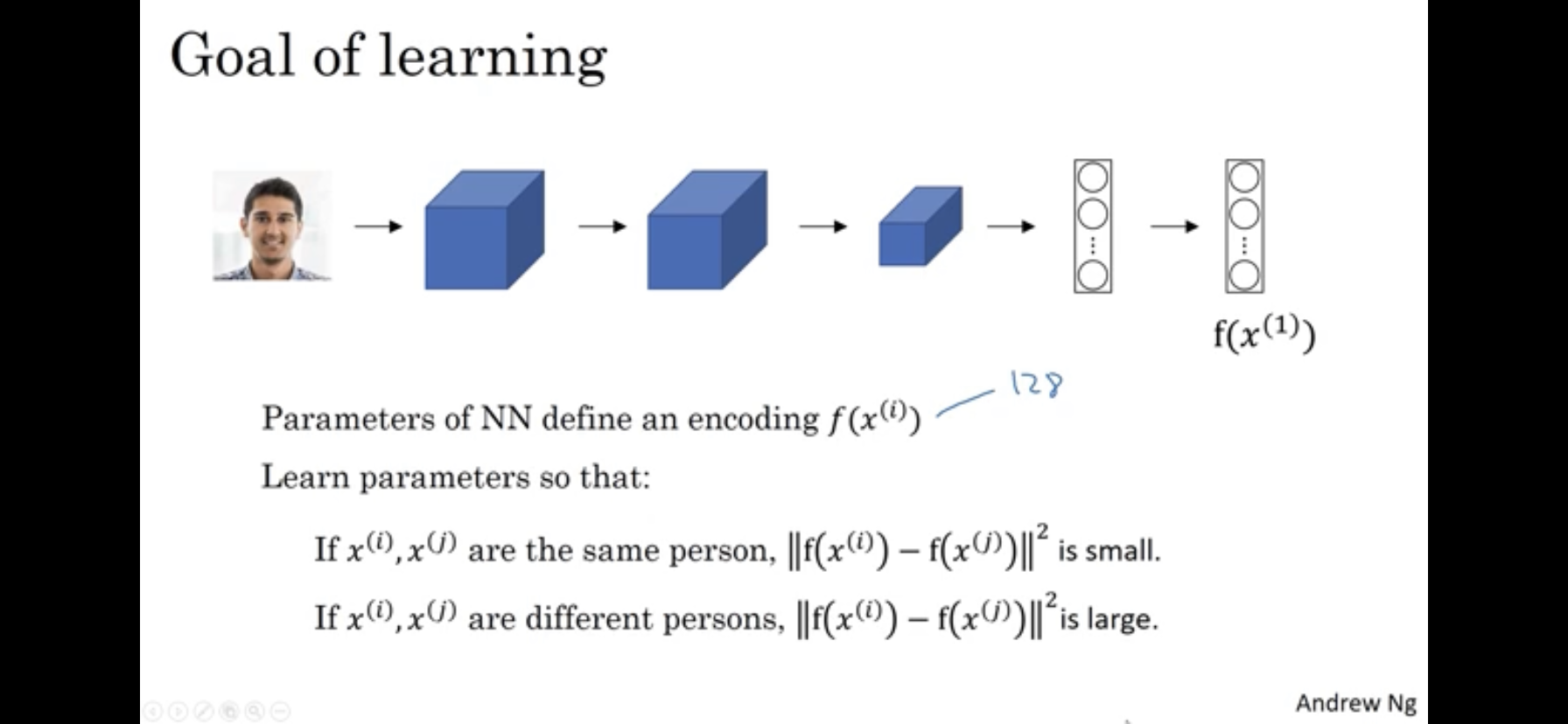
• A pair of pictures \(x^{(i)}, x^{(j)}\) are fed to the same neural network. The goal is for the network to learn to differentiate them if they are different or similar.

Principal Component Analysis

Summary. The principal components of a collection of points in a real coordinate space are a sequence of $p$ unit vectors, where the $i$-th vector is the direction of a line that best fits the data while being orthogonal to the first $i-1$ vectors. Thus, the first vector is the line that best fits the data, while the second vector is the second best line while being orthotogonal to the first, etc.

Motivation. PCA is often used for dimensionality reduction. We can reduce from $n$ dimensions to $k$ by selecting only the first $k$ principal components.

Algorithm. Calculate mean of all values. Shift data such that mean is at the origin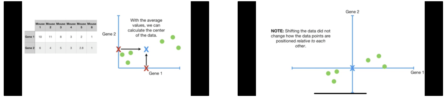

Find the first principal component (PC1). That is, start by drawing a random line through the origin. Slowly rotate such that it either 1) minimizes distances from the data to the line or 2) maximises the distances from the projected points to the origin. The two are equivalent because of pythagoras theorem. Let distance between point and origin be c, distance between point and line be a, and projection of point to line be b. Since $c^2 = a^2 + b^2$ (by pythagoras theorem) and $c^2$ is constant, minimising a is same as maximizing b.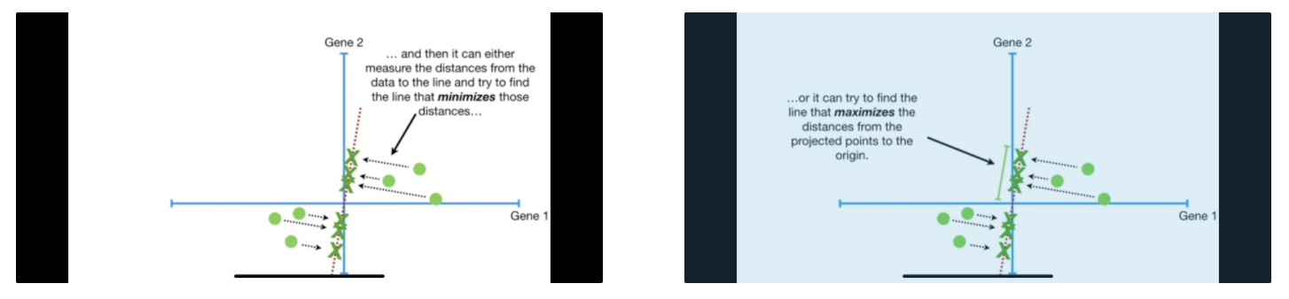

Next, find PC2, the next best fitting line given that it goes through the origin and is perpendicular to PC2. Repeat steps 1 and 2 until $k$.

Suppose $k=2$. Project samples onto PC1 and PC2. Compute PCA plot based on projected samples.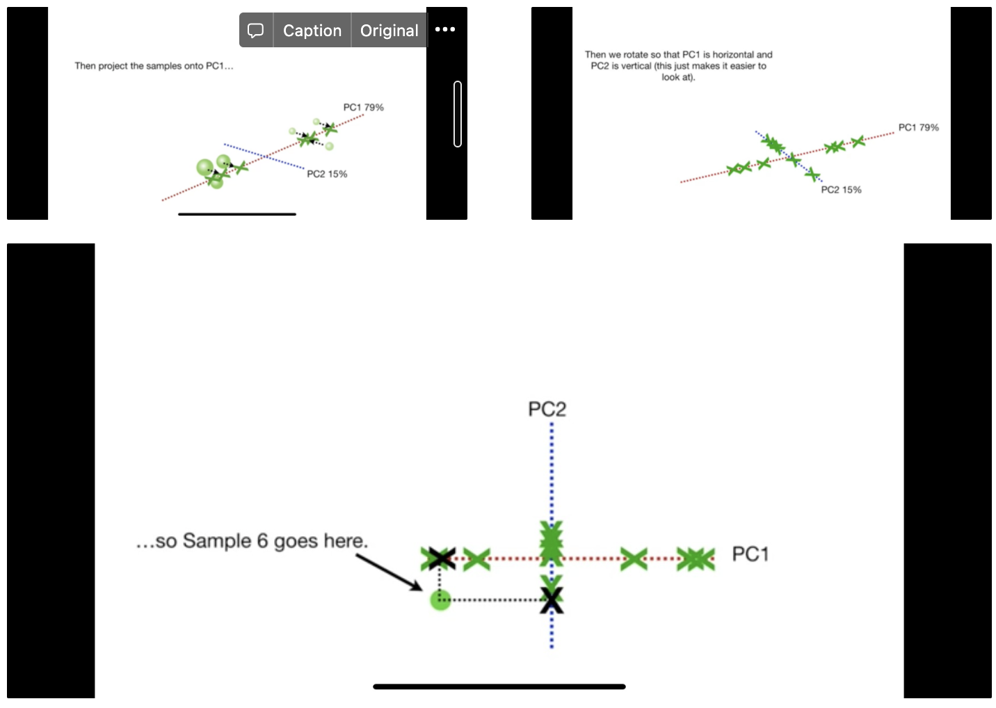

How to evaluate each principal components? Compute the sum of squared distances (SS) for the principal component. From point 2 of the algo, the larger this distance, the better. Thereafter, compute the variation and plot the scree plot. From the example below, limiting to two dimensions is good enough.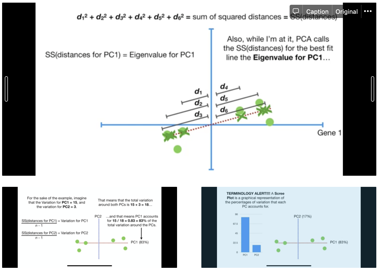

How to reconstruct plots for principle components? For each point, project them to each principle component. Reconstruct plot from the remaining principle components. For example, if there are two principle components left (x and y-axis), then the sample which is on -1 on the x axis and 1 on the y-axis will take the point (-1, 1).

Thanks Statquest for the explanation! Link here.

Kullback–Leibler divergence (KL divergence). The KL divergence, $D_{KL}(P \Vert Q)$, is a numerical measure of the distance between two probability distributions. For example, consider the following distributions:

We are interested in the distance between the distributions of $X$ and $Y$. Suppose $p=0.5, q=0.1$, we can tell quite obviously that $Y$ is different from $X$ by simply sampling from $X$. But how do we quantify this distance?

We can gauge this distance by computing the likelihood ratio:

If the distributions are similar, then the ratio should equal 1. The KL divergence builds on via:

This now follows the more general form (which you can refer to wiki for):

Some properties:

1. $D_{KL}(P \Vert Q) \geq 0$
2. $D_{KL}(P \Vert Q) = 0$ if $P = Q$ almost everywhere.

Thanks to this awesome youtube channel for the explanation! Link here.

NLP

Word2Vec The motivation is to turn each to vectors. There are two primary algorithms to do so: CBOW and Skip-Gram. CBOW tries to predict a center word from the surrounding context. For each word, we learn two vectors: 1) v (input vector), when the word is in the context and 2) u (output vector), when the word is in the center. Skip-Gram tried to predict the surrounding word from the given center word.

Training Word2Vec algorithms are expensive due to the large vocabulary size. Specifically, optimising the cost function and the softmax operator both involves looping through the vocabulary. We use negative sampling to circumvent the first problem and hierarchical softmax for the second.

Math

Taylor Series(3Blue1Brown)

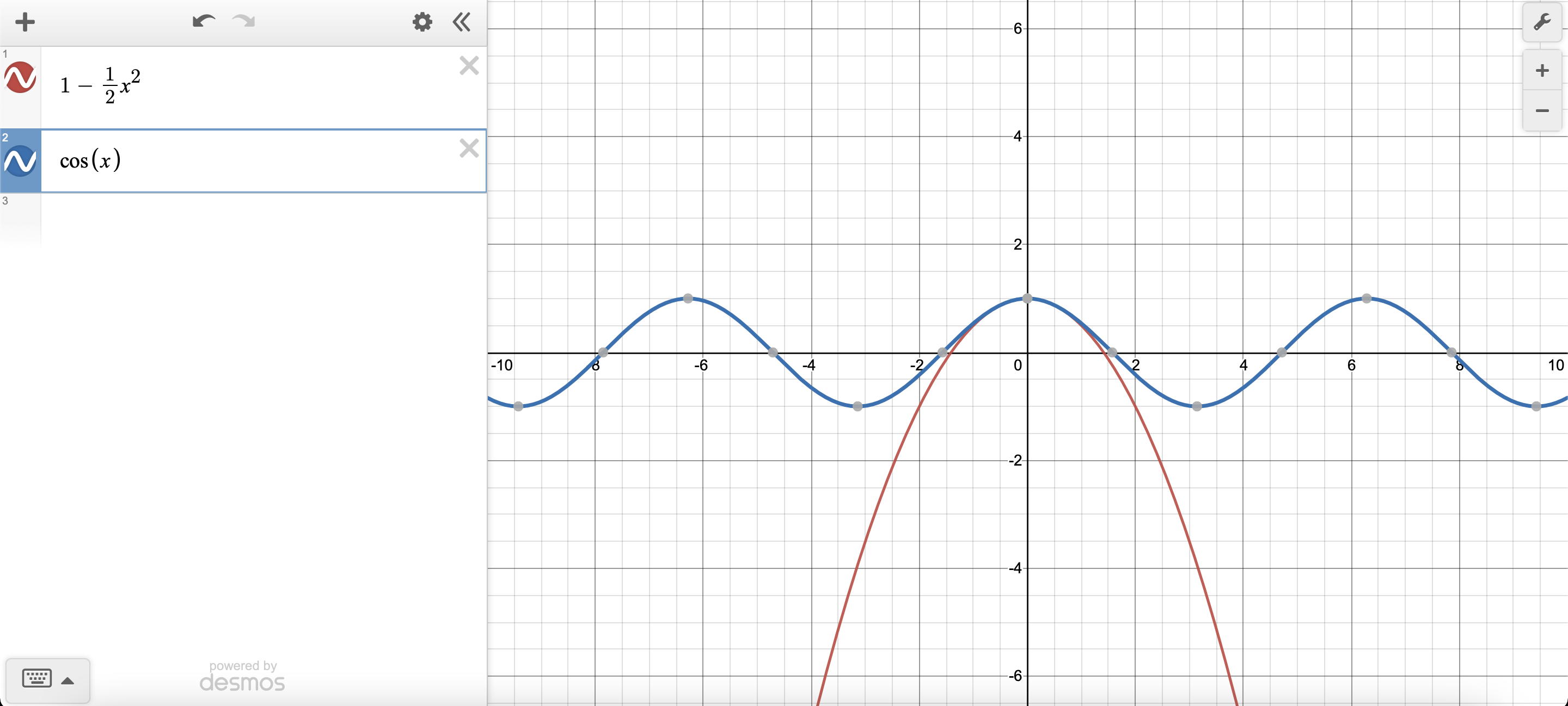
Motivation. To approximate non-polynomial function as a polynomial. Polynomials are in general easier to deal with (easier to compute, obtain derivatives etc).

Concretely, consider the problem of approximating $cos(x)$ as a polynomial $P(x) = c_0 + c_1 x + c_2 x^2$. We can approximate them by ensuring their derivatives at $x=0$ are the same.

To ensure their derviatives at $x=0$ are the same,

Thus, $cos(x) \approx 1 - \frac{1}{2} x^2$. Notice how every derivative order is independent of each other and provides a unique information (i.e. $P(0)$ provides the intersection point, $P’(0)$ provides the correct gradient, $P’‘(0)$ provides the correct rate etc.)